Course: MT-2002 Statistical Modeling Fall 2026 Student ID: i222327

Bayesian Statistical Modeling with PyMC

Campus service-center case study: estimate daily demand, model resolution times under an outlier, compare Poisson/ZIP and Gaussian/Student-t models, then turn posterior inference into ROPE, staffing, and SLA decisions.

Open operations dashboard Full notebook report GitHub repository

Live Link

Official project entry points with clean, readable URLs.

Project overview

Completed MT-2002 Assignment 1 notebook with a full professional extension layer for portfolio and viva defense.

Business question

How many requests arrive on a typical day, and how long do selected requests take to resolve?

Data

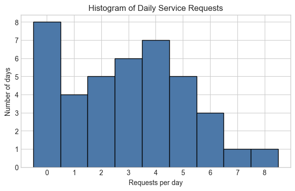
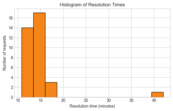
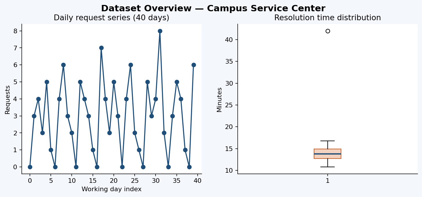
40 daily request counts and 35 resolution times, including one unusual 42-minute observation.

Method

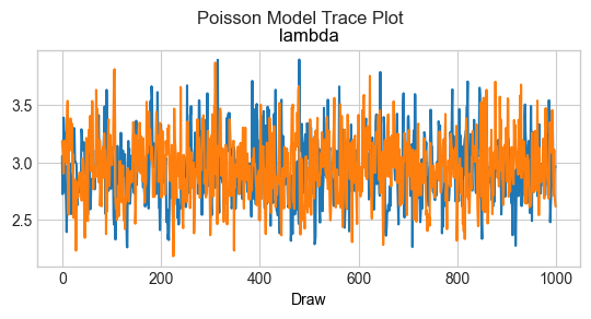
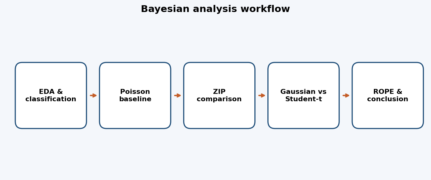
Bayesian priors, MCMC (2 chains), 94% HDIs, PPC, LOO, ROPE, utility, and calibration tools.

Assignment depth — what was required and what we delivered

Interactive case accordion. Open any case to see the required task and the delivered analysis.

Case 1 — Understanding the data

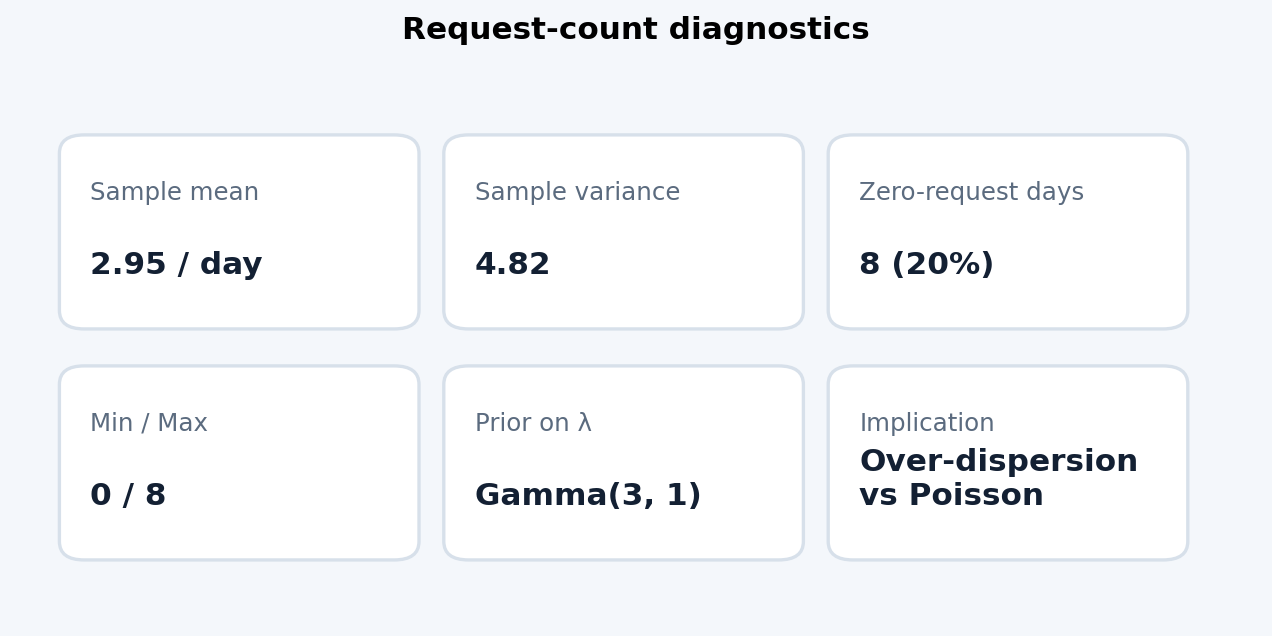
Classify discrete vs continuous variables, compute diagnostics, and produce exploratory histograms for demand and resolution time.

Case 2 — Poisson demand model

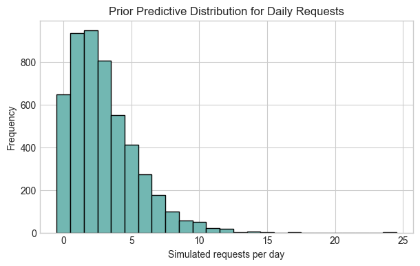
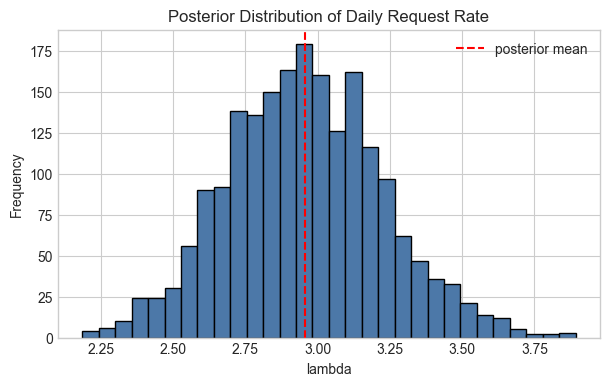
Specify Gamma prior for λ, check prior predictive distribution, sample posterior, report mean and 94% HDI.

Case 3 — Zero-inflated Poisson

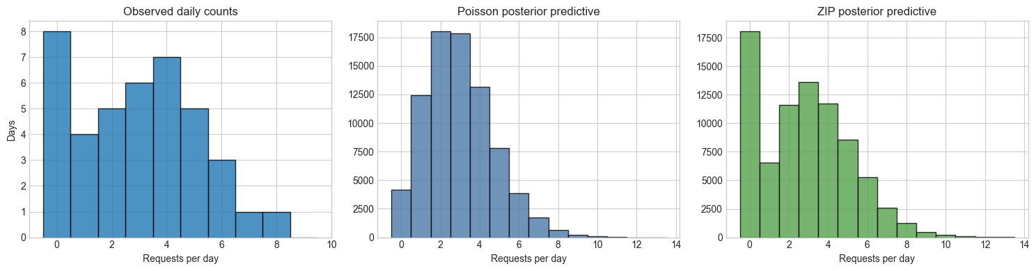
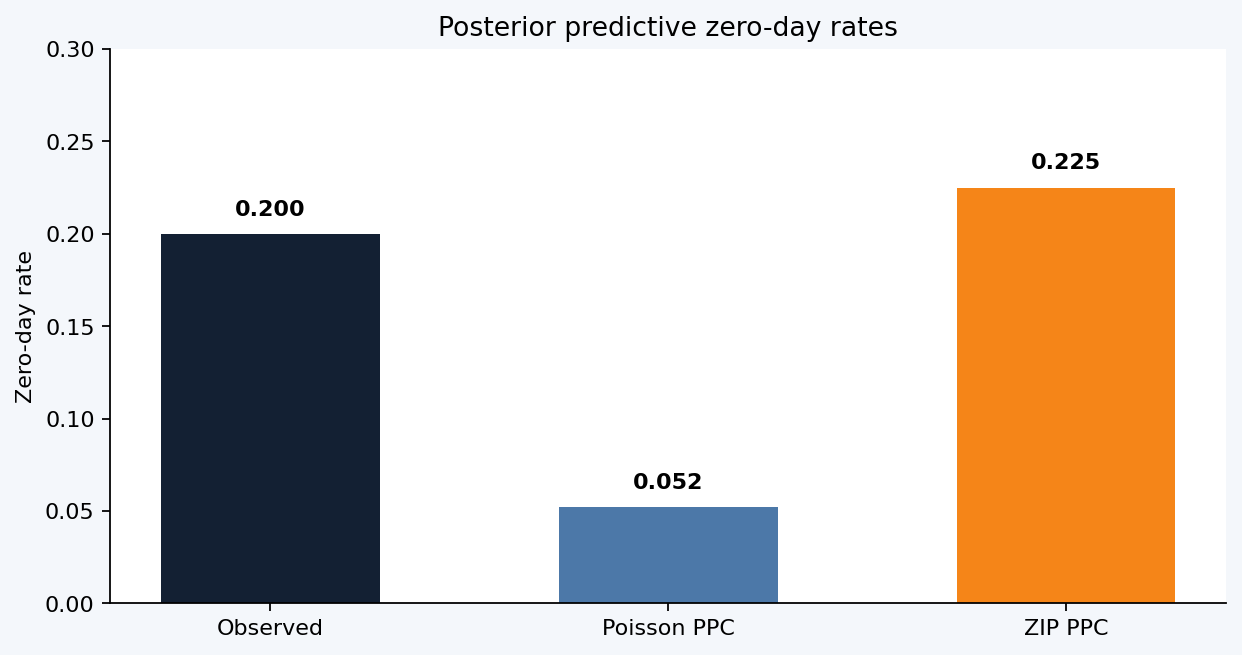
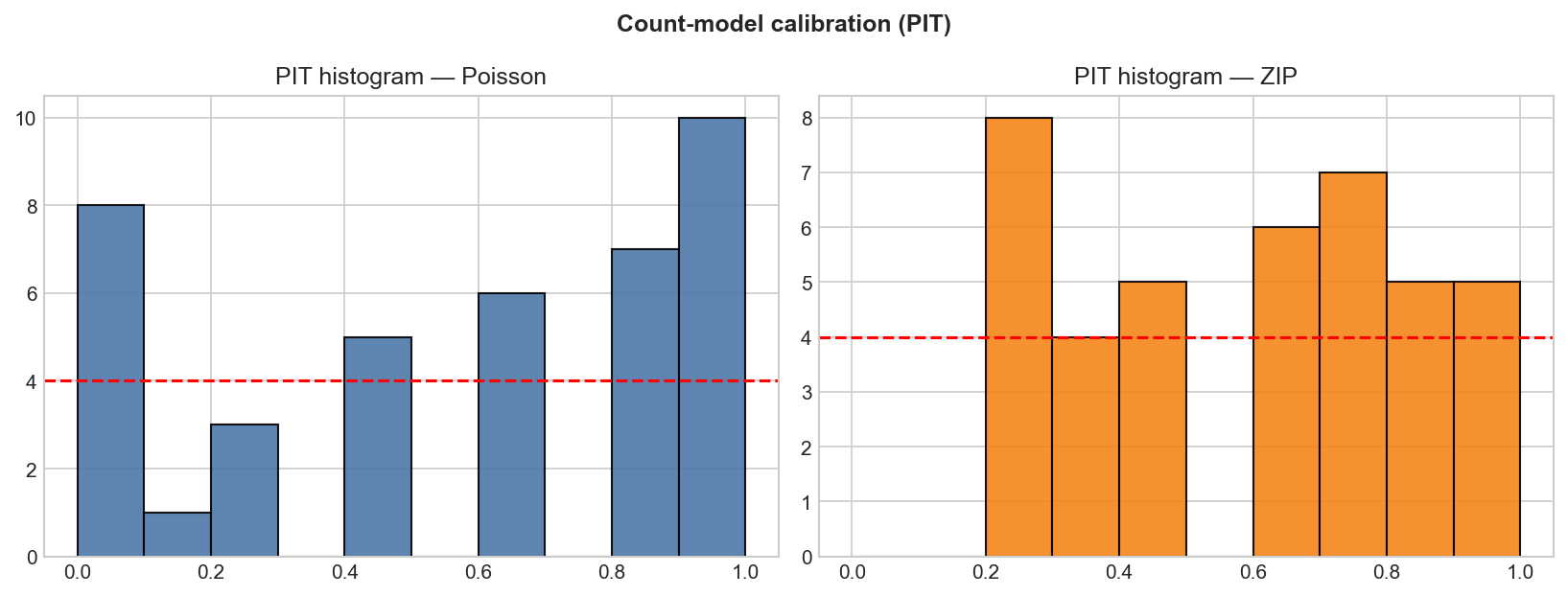
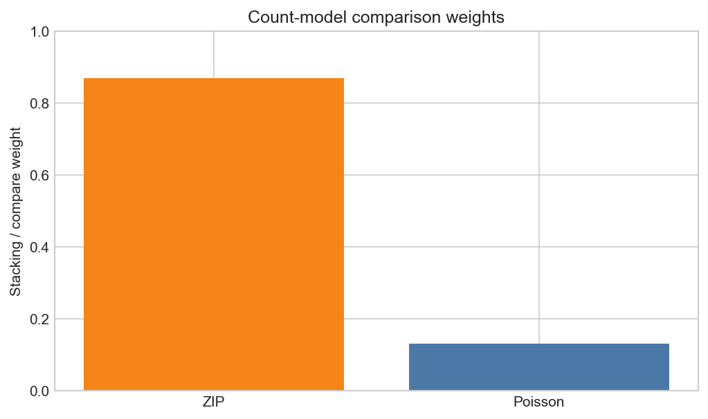
Test whether zero-request days need a separate process; compare Poisson vs ZIP with PPC zero-day rates.

Cases 4–6 — Resolution-time models

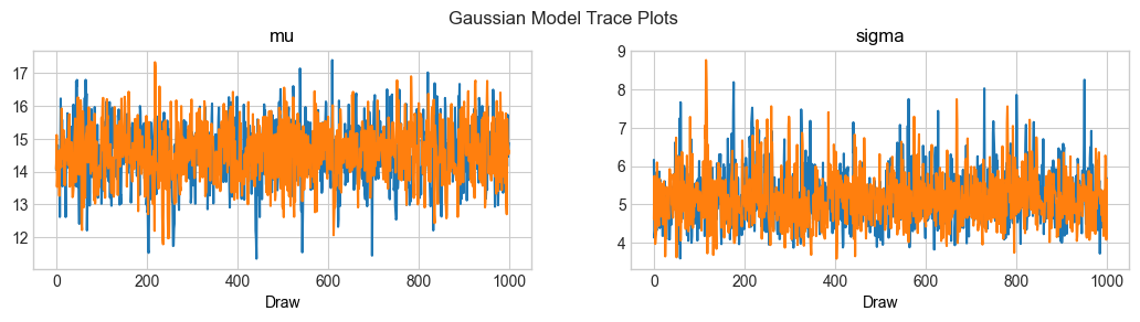
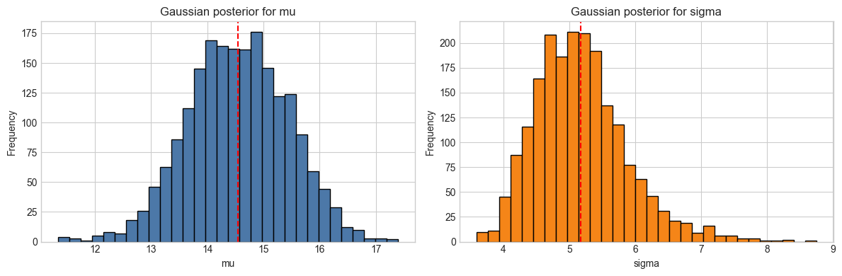
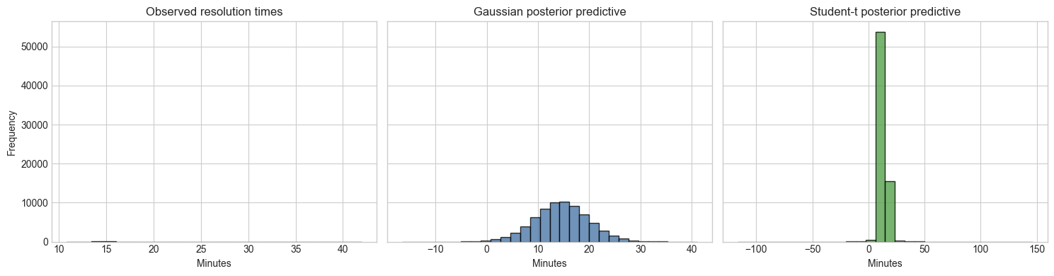
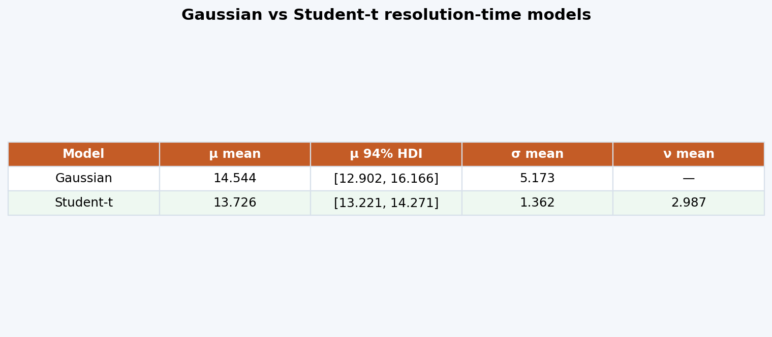
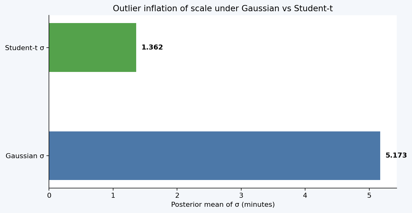
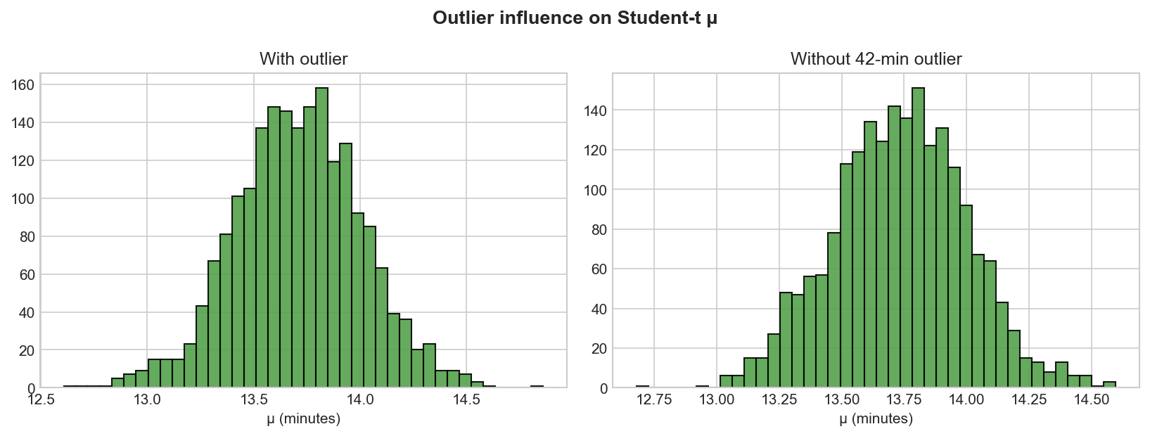
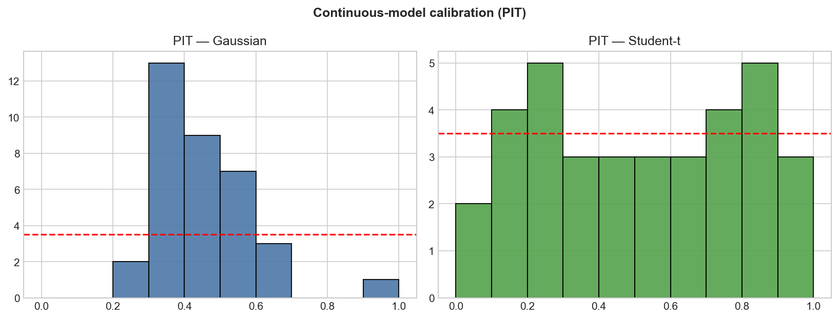
Fit Gaussian and Student-t models, compare parameters and predictive fit, explain outlier influence of the 42-minute case.

Cases 7–8 — ROPE and integrated decision

Compare μ against a 14-minute operational benchmark using ROPE rules, then write a management-facing conclusion.

Extension Packs A–C — Cases 9–30

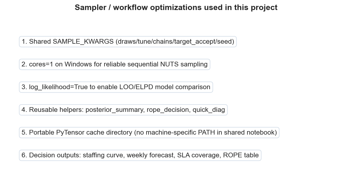
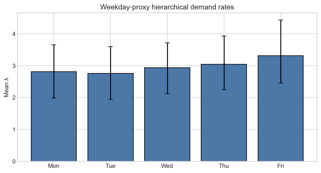
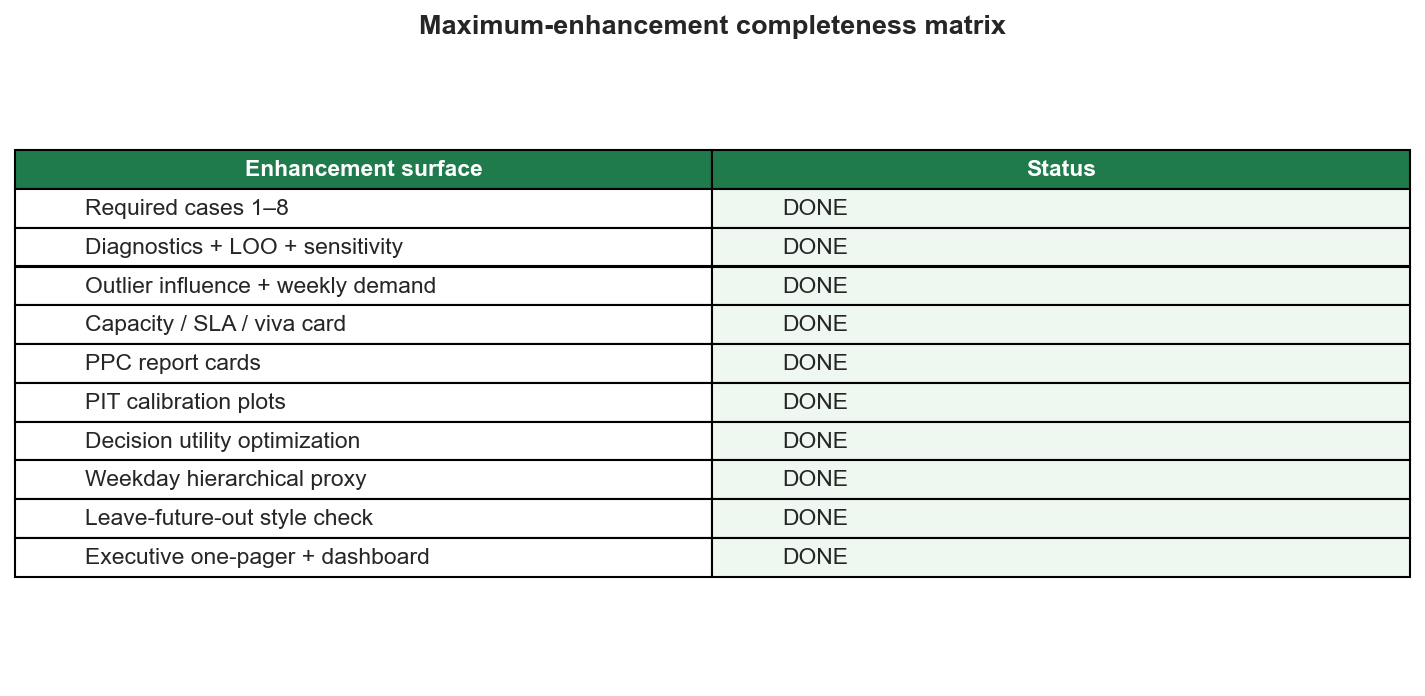
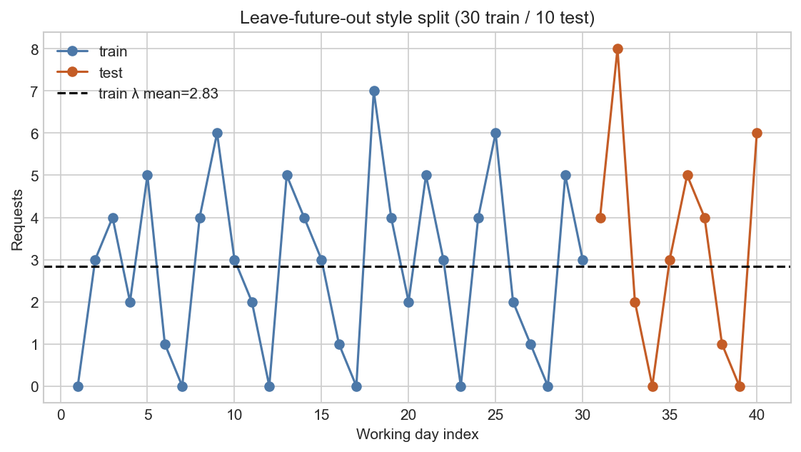
Diagnostics, LOO, sensitivity, influence, staffing/SLA tools, PIT calibration, utility optimization, hierarchical weekday proxy, leave-future-out check, and saturation board.

Models fitted

Switch tabs to inspect count models, continuous models, and decision tools.

Poisson(λ)

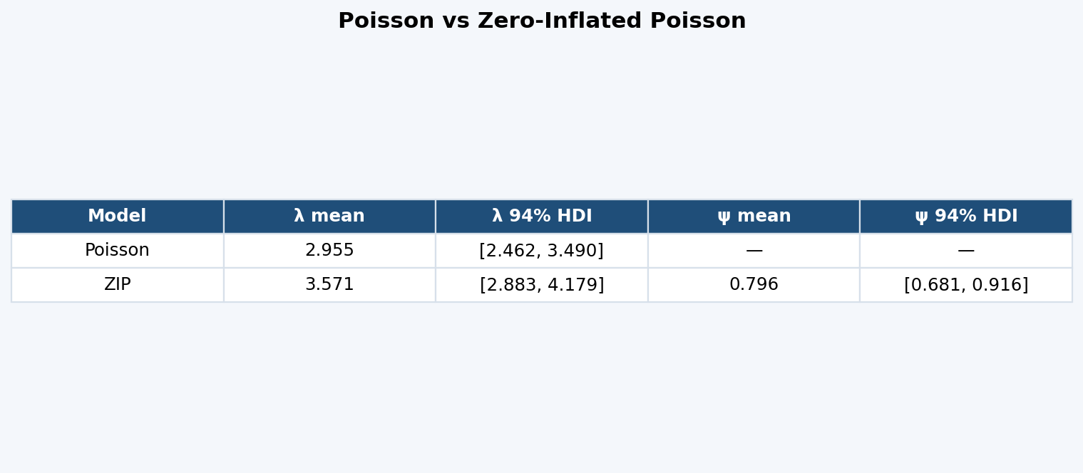
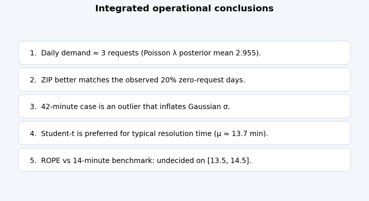
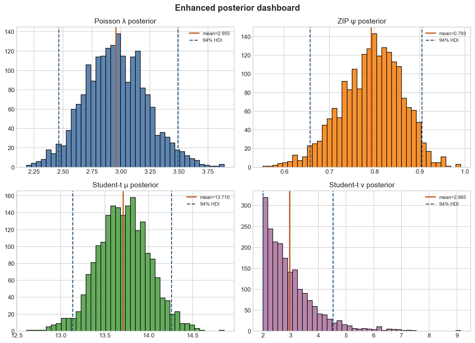
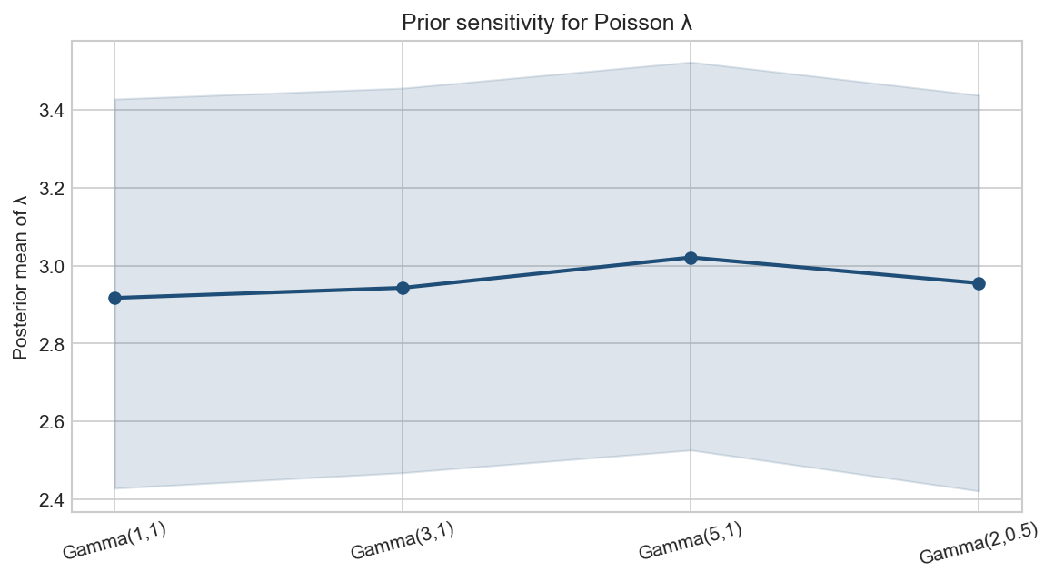
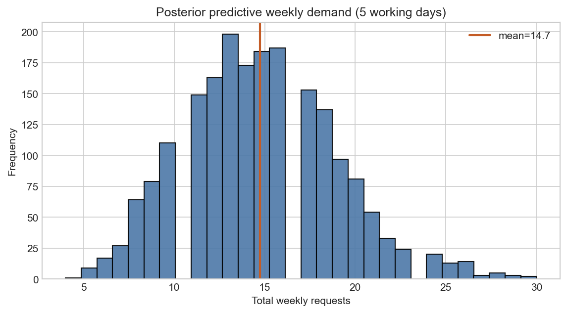
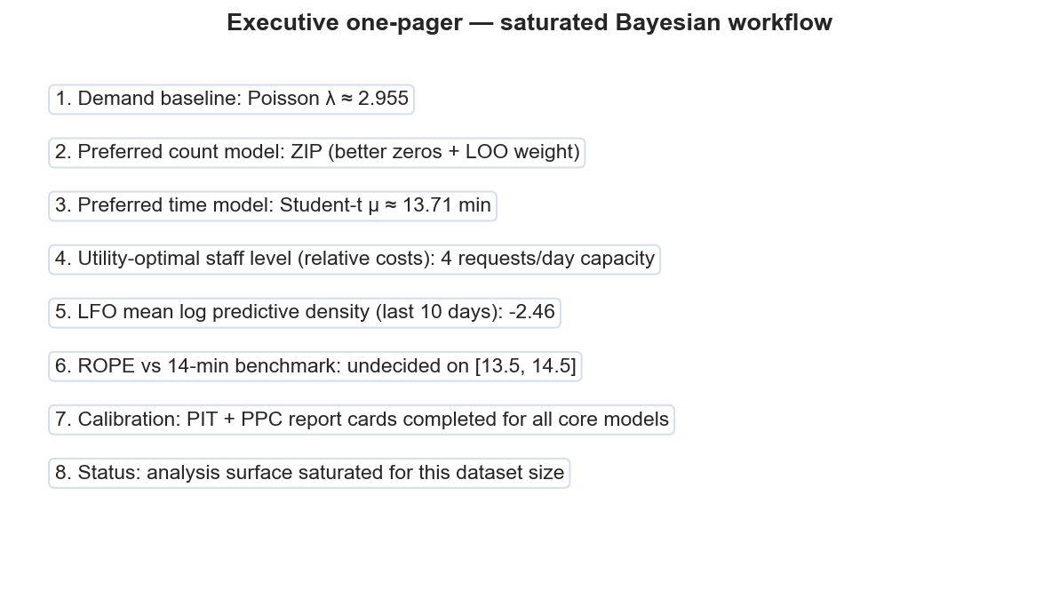
Gamma(3,1) prior. Baseline daily demand model with posterior λ ≈ 2.955.

Zero-Inflated Poisson

Beta(2,2) on ψ and Gamma on λ. Recovers the observed 20% zero-day rate.

Gaussian

Sensitive to the 42-minute outlier; σ inflates to about 5.2 minutes.

Student-t

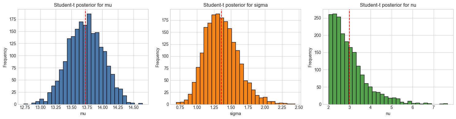
Preferred model for typical time: μ ≈ 13.71, σ ≈ 1.36, ν ≈ 2.97.

ROPE

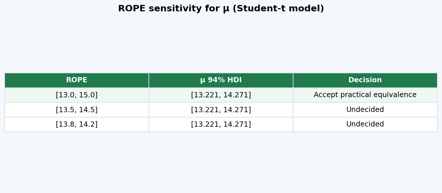
Against 14 minutes, default ROPE [13.5, 14.5] remains undecided.

Utility & SLA

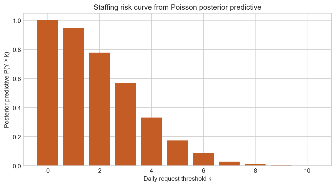
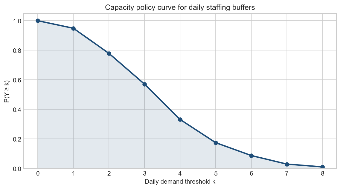
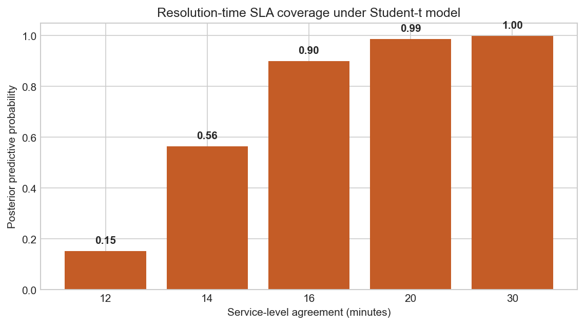
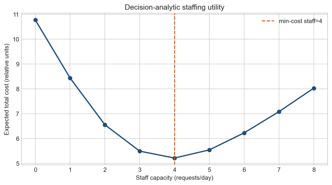
Staff optimum = 4 under relative costs; SLA coverage curves for 12–30 minutes.

Selected numerical results

Values from the executed notebook outputs (seed 2026).

Quantity	Estimate	Interpretation
Request mean / variance	2.95 / 4.82	Over-dispersion vs pure Poisson
Poisson λ posterior	2.955 · HDI [2.462, 3.490]	Baseline expected daily demand
ZIP ψ / λ	0.793 / 3.570	Extra zero process improves quiet-day fit
Gaussian μ / σ	14.517 / 5.157	Outlier inflates center and scale
Student-t μ / σ / ν	13.710 / 1.359 / 2.965	Preferred continuous model
Utility-optimal staff	4	Minimum expected relative cost

Full traces, predictive plots, comparison tables, and discussion are in the HTML report and source notebook.

Visual gallery

Filter by pack or search captions. Headings sit above every screenshot.

**01 · Case 1 — Requests histogram**Discrete demand across 40 working days.

**02 · Case 1 — Resolution histogram**Includes the 42-minute outlier.

**03 · Case 2 — Prior predictive**Poisson prior predictive counts.

**04 · Case 2 — Poisson trace**MCMC diagnostics for λ.

**05 · Case 2 — Poisson posterior**Posterior density for daily demand rate.

**06 · Case 3 — Count PPC**Observed vs Poisson/ZIP predictions.

**07 · Case 4 — Gaussian traces**Diagnostics for μ and σ.

**08 · Case 4 — Gaussian posteriors**Normal-error parameter uncertainty.

**09 · Case 5 — Student-t posteriors**μ, σ, and ν under heavy tails.

**10 · Case 6 — Continuous PPC**Gaussian vs Student-t predictive fit.

**11 · Cases 1–8 — Dataset overview**Series + boxplot briefing board.

**12 · Case 1 — Count diagnostics**Mean, variance, zero-day summary.

**13 · Case 3 — Poisson vs ZIP**Posterior means and 94% HDIs.

Zero-day rates — **14 · Case 3 — Zero-day PPC rates**ZIP recovers the 20% quiet-day rate.

**15 · Case 6 — Continuous comparison**Gaussian vs Student-t table.

**16 · Cases 5–6 — Outlier scale effect**Gaussian σ inflation vs Student-t.

**17 · Case 7 — ROPE sensitivity**Practical equivalence around 14 minutes.

**18 · Cases 1–8 — Workflow**EDA to ROPE conclusion path.

Conclusions — **19 · Case 8 — Key conclusions**Operational takeaways board.

Stack — **20 · Reproducibility stack**Libraries, delivery, seed.

Dashboard — **21 · Pack A — Posterior dashboard**λ, ψ, μ, ν stakeholder board.

**22 · Case 11 — Prior sensitivity**λ stability across Gamma priors.

**23 · Case 13 — Staffing risk**Daily exceedance probabilities.

**24 · Case 13 — Weekly forecast**Five-day total demand distribution.

**25 · Case 12 — Outlier influence**Student-t μ with/without 42-min case.

**26 · Case 16 — Capacity policy**Staffing-buffer policy curve.

**27 · Case 17 — SLA coverage**Minute-based service-target probabilities.

**28 · Case 19 — Optimization checklist**Sampler/workflow reproducibility board.

**29 · Case 22 — PIT counts**Calibration for Poisson vs ZIP.

**30 · Case 22 — PIT continuous**Calibration for Gaussian vs Student-t.

Utility — **31 · Case 23 — Staffing utility**Relative-cost optimum at staff = 4.

**32 · Case 24 — Weekday rates**Hierarchical day-type demand proxy.

Weights — **33 · Case 26 — Model weights**ZIP vs Poisson predictive weights.

**34 · Case 28 — Executive one-pager**Saturated workflow summary.

**35 · Case 29 — Completeness matrix**Saturation declaration.

LFO — **36 · Case 25 — Leave-future-out**Chronological 30/10 train-test split.

How to run locally

Create a virtual environment, install dependencies, and open the notebook.

python -m venv .venv
.venv\Scripts\activate
pip install -r requirements.txt
jupyter notebook notebook/i222327_A01_A_SM.ipynb