Step metrics
Rise time uses the first threshold crossings. Peak and settling time depend on the simulation grid. A null settling time means the window did not establish settling.
Step response, stability margins, and gain sensitivity for a PI-controlled plant.







| What | Link |
|---|---|
| Repository | https://github.com/rohaan2802/PI_Control |
| GitHub Pages | https://rohaan2802.github.io/PI_Control/ |
| SciPy LTI reference | https://docs.scipy.org/doc/scipy/reference/signal.html#continuous-time-linear-systems |
A Python study of a proportional–integral controller for the damped plant G(s) = 1/[s(s + 2)]. It examines reference tracking, closed-loop stability, and open-loop frequency margins.
| Resource | Link |
|---|---|
| Analysis and CLI | pi_control/__main__.py |
| Plot exporters | pi_control/plots.py |
| Verification notes | docs/verification.md |
| Dependencies | requirements.txt |
| Website preview | index.html |
Under negative unity feedback, L(s) = (Kp s + Ki)/[s²(s + 2)] and T(s) = (Kp s + Ki)/(s³ + 2s² + Kp s + Ki). With positive gains, the Routh array gives Ki < 2 Kp. The controller zero is −Ki/Kp.
The original gains are Kp = 2.02488613 and Ki = 0.06465480. The 160 s simulation gives 1.441 s rise time, 7.738% overshoot, 16.29 s settling time, and 63.303° phase margin. The stable closed-loop DC gain is one. Gain margin is infinite for the baseline loop.
Rise time uses the first 10% and 90% crossings of the unit reference, with interpolation between samples. Overshoot is measured relative to the unit target. Settling uses the last sample outside the ±2% band. Steady-state error comes from DC gain. Stability margins come from the open loop, while closed-loop magnitude and phase describe reference tracking.
Rise time uses the first threshold crossings. Peak and settling time depend on the simulation grid. A null settling time means the window did not establish settling.
The last simulated point depends on the duration. For a stable system the analytical final value is one, so the unit-step tracking error tends to zero.
The Routh first column is 1, 2, (2 Kp − Ki)/2, Ki. At Ki = 2 Kp the poles include an imaginary-axis pair.
The gallery holds one gain fixed while sweeping the other. It also shows the poles and unit-step responses around the Routh boundary. These sweeps illustrate sensitivity to the gains. They do not automate controller tuning.
This model assumes a linear continuous-time plant, ideal feedback, a unit step, and zero initial conditions. There is no hardware validation. Finite sampling limits peak and settling-time precision, especially near the stability boundary.
Change Kp and the fraction Ki / (2 Kp). At a fraction of 1 the poles reach the imaginary axis. Above 1 the nominal linear model is unstable.
The browser integrates the ideal model for 30 seconds. Use the Python CLI and a longer horizon for settling estimates.
Filter by topic or search captions. Open a figure to inspect the full frame.
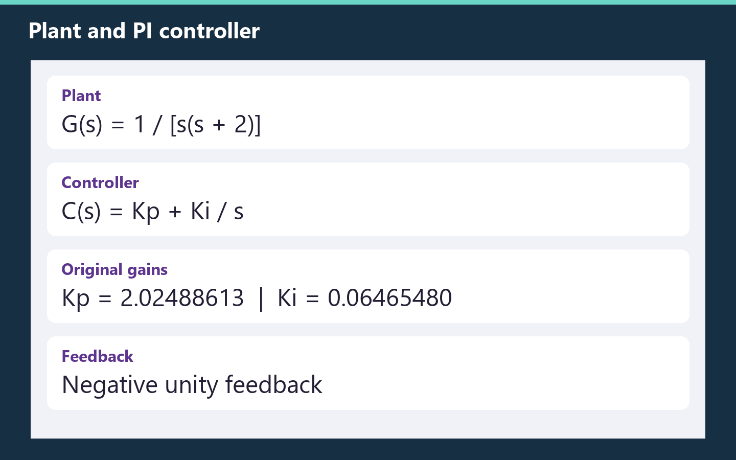
Continuous-time transfer functions from the original assignment.
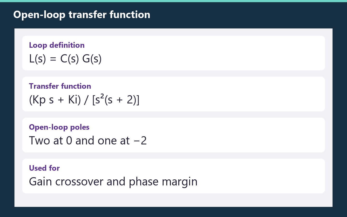
The loop combines the controller and plant. Its response determines the stability margins.
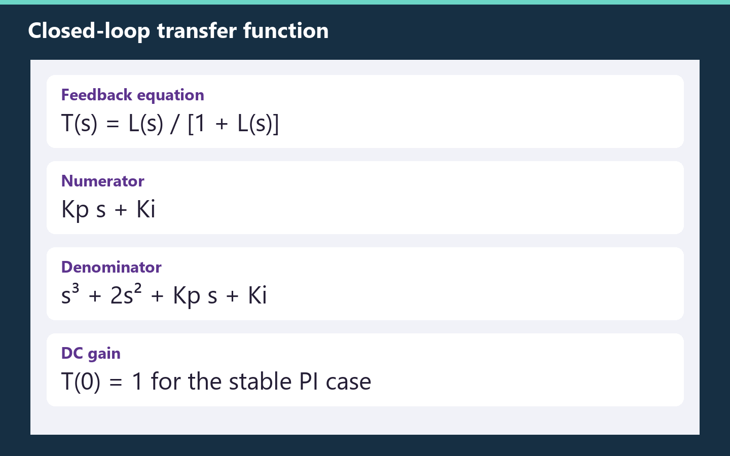
Unity feedback gives a third-order characteristic polynomial.
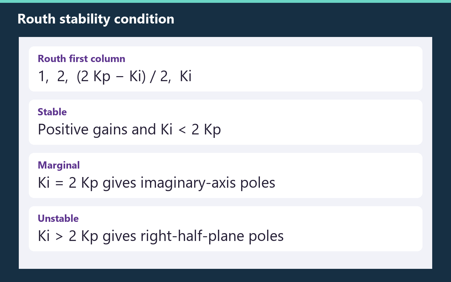
For positive gains, strict stability requires Ki < 2 Kp.
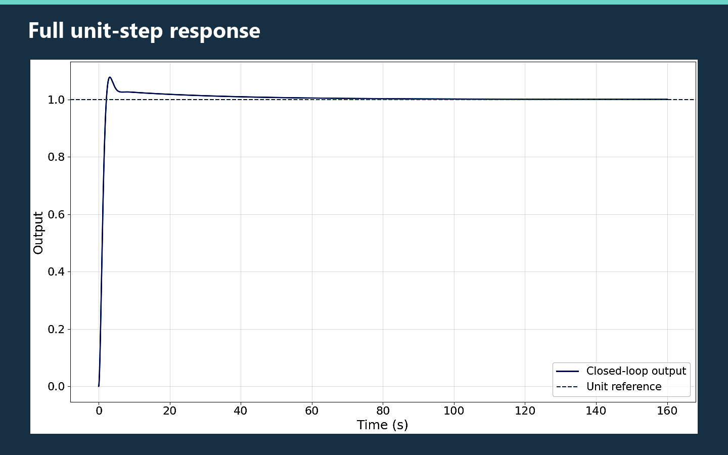
The long horizon shows the slow approach to the analytical final value.
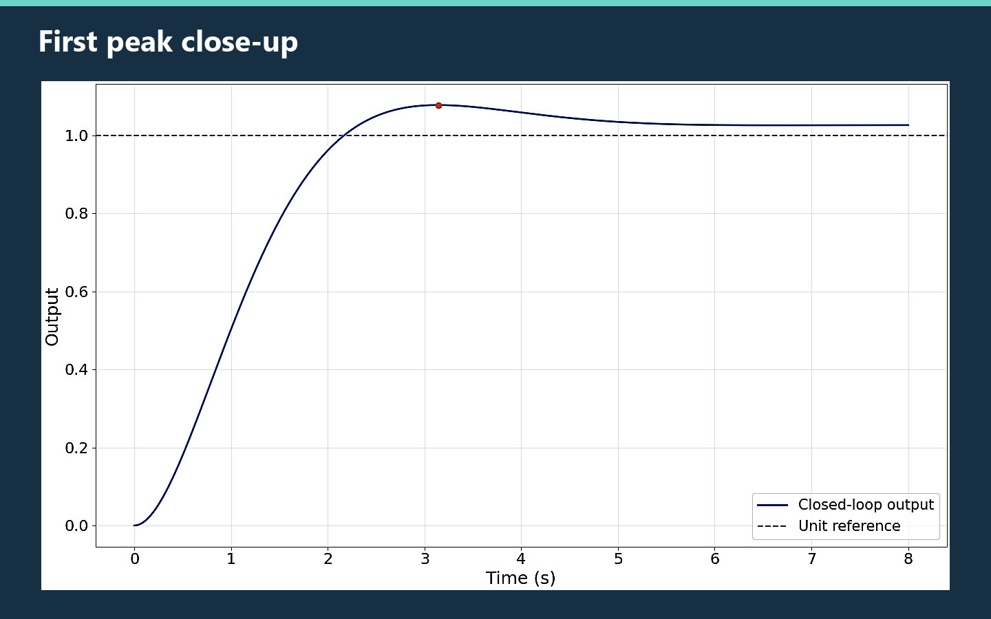
The baseline peak occurs at about 3.14 s.
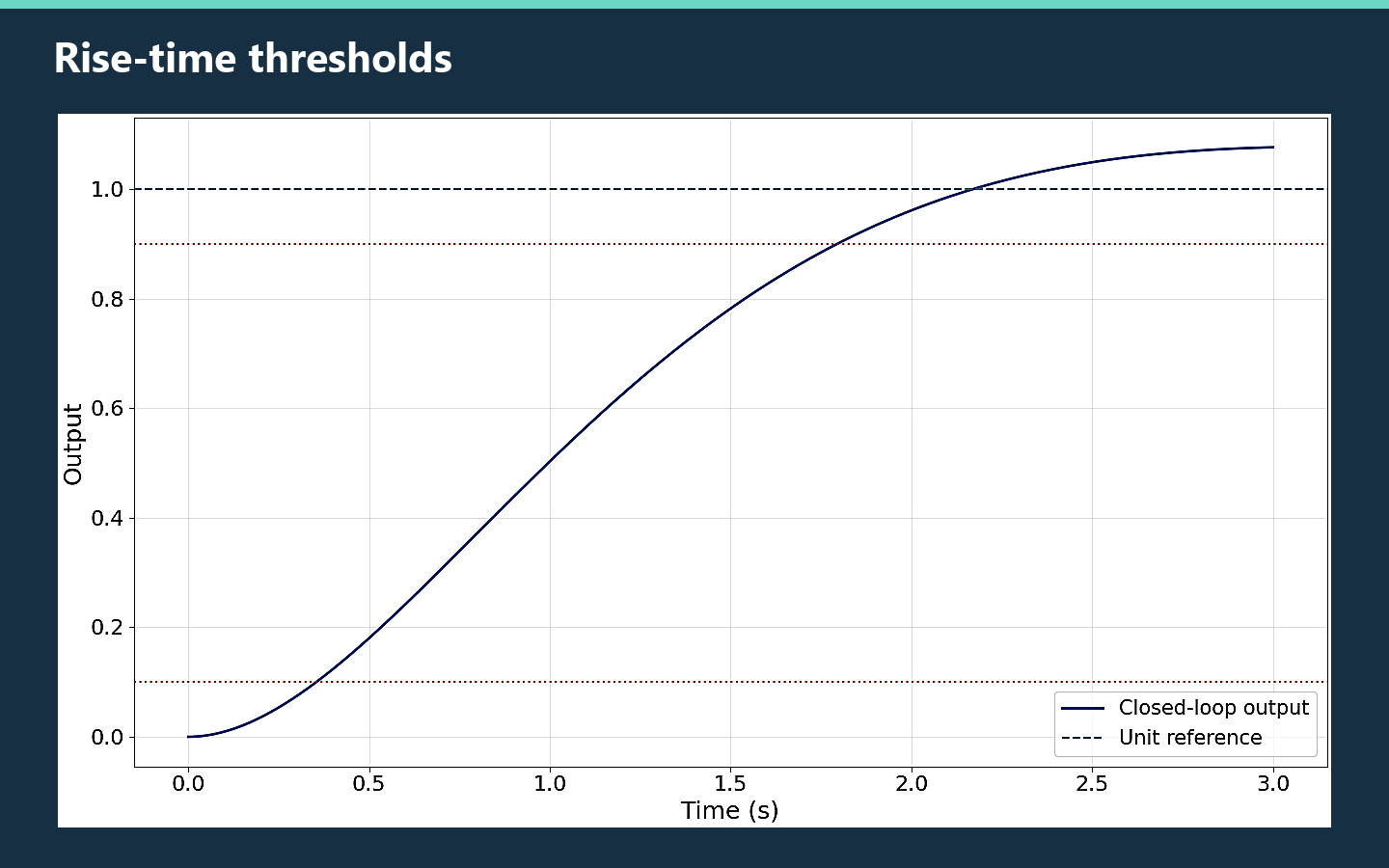
The first crossings of 0.1 and 0.9 define the 10–90% rise time.
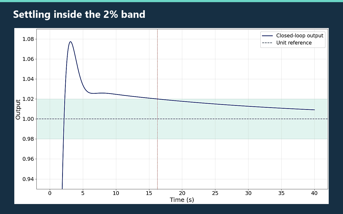
The estimated settling time is 16.29 s on the baseline grid.
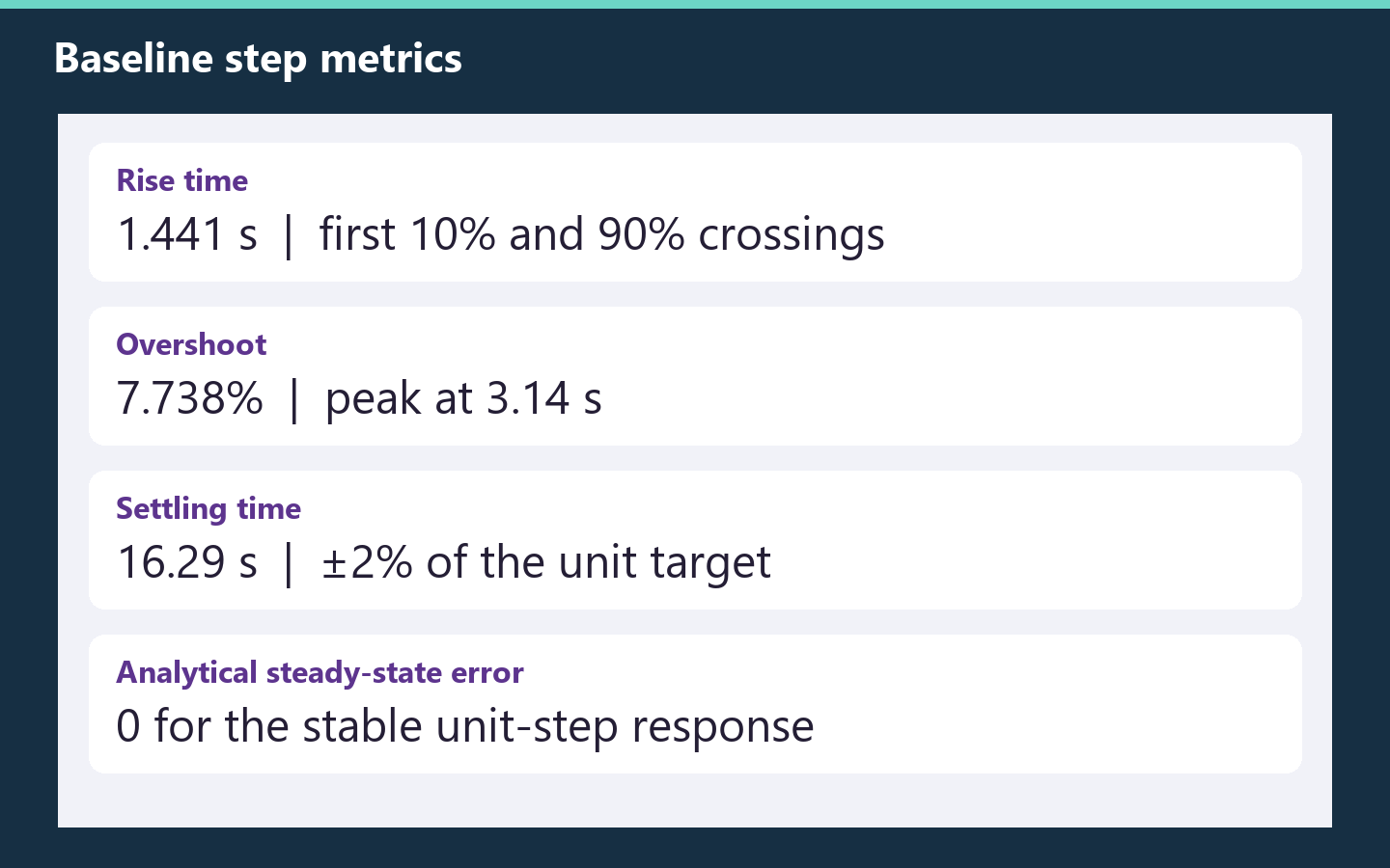
Metrics use the unit target as the steady-state value.
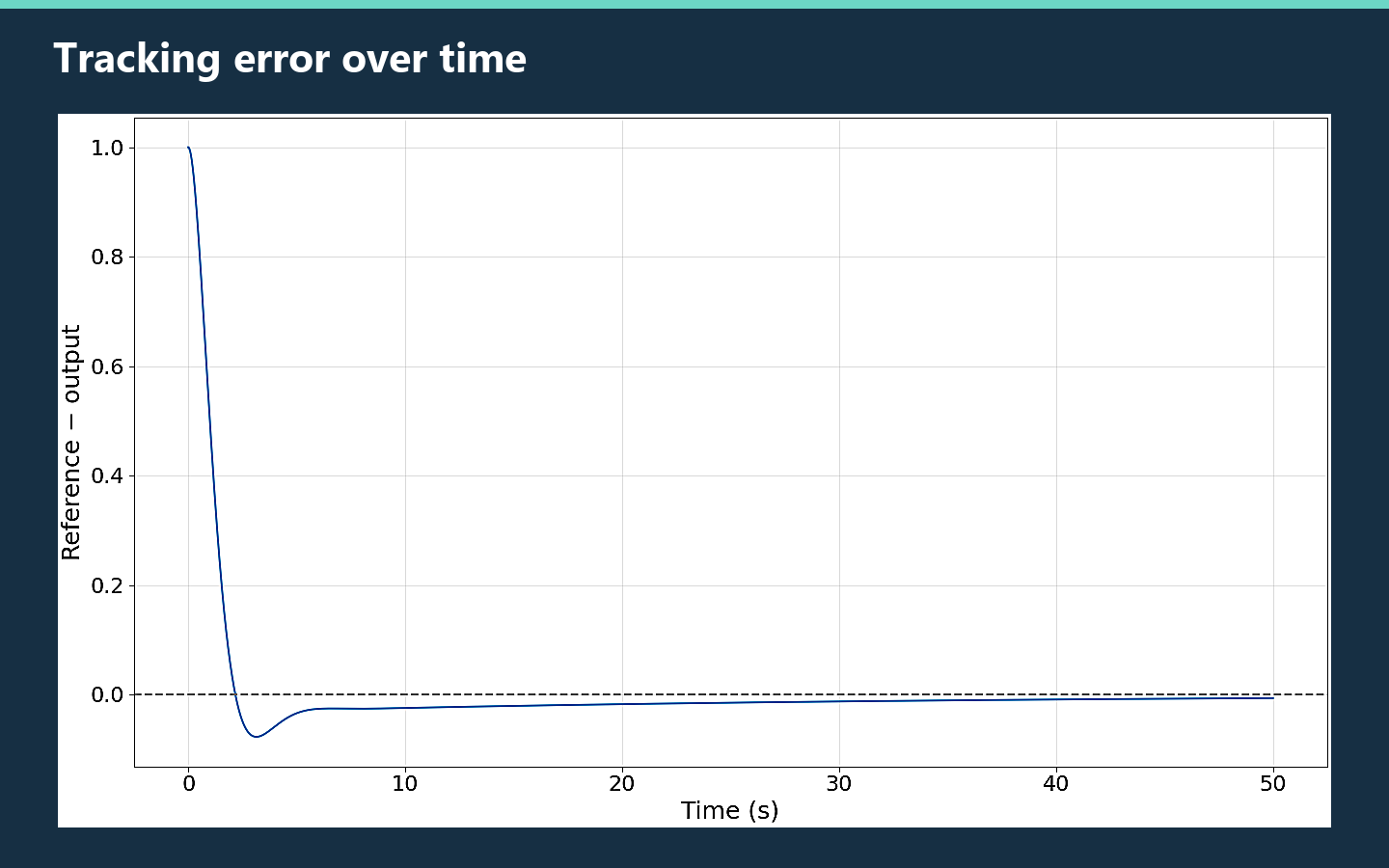
The signed difference between the unit target and the output.
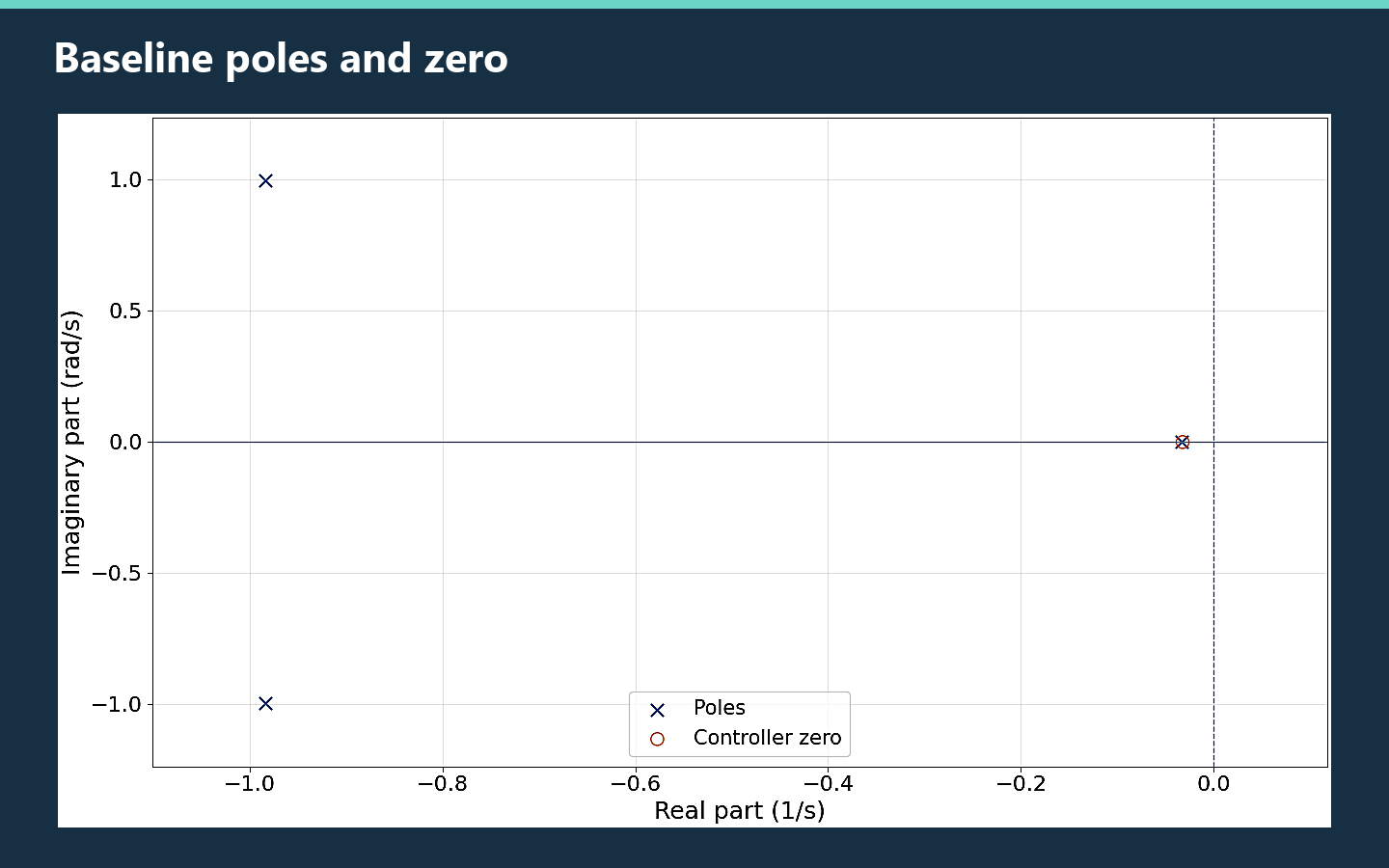
The three poles lie in the left half-plane.
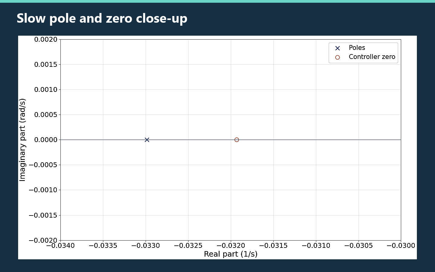
The real pole and controller zero are close together but distinct.
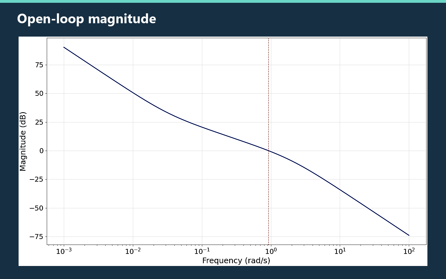
The gain crossover is where the open-loop magnitude reaches 0 dB.
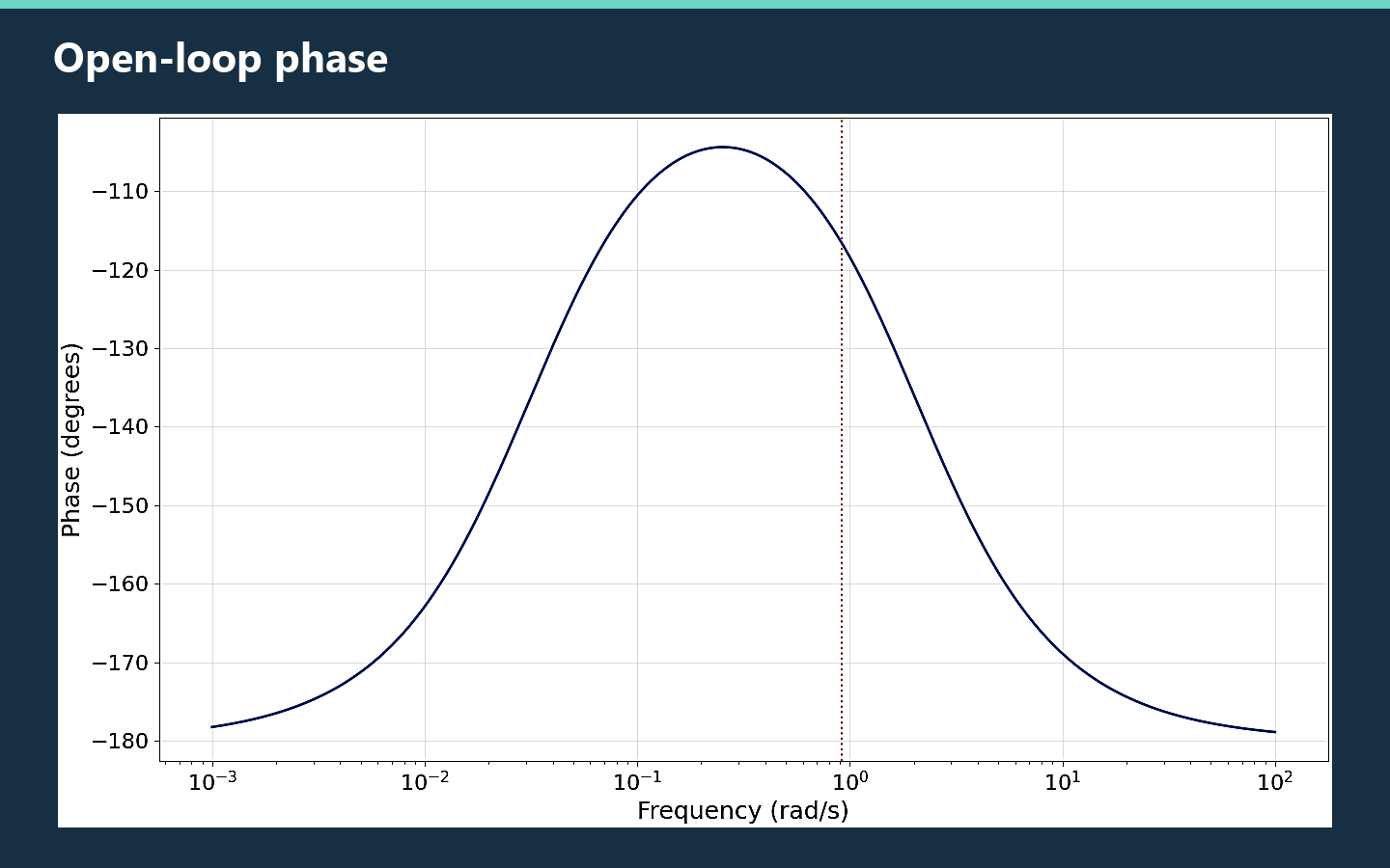
The open-loop phase is evaluated at gain crossover to obtain phase margin.
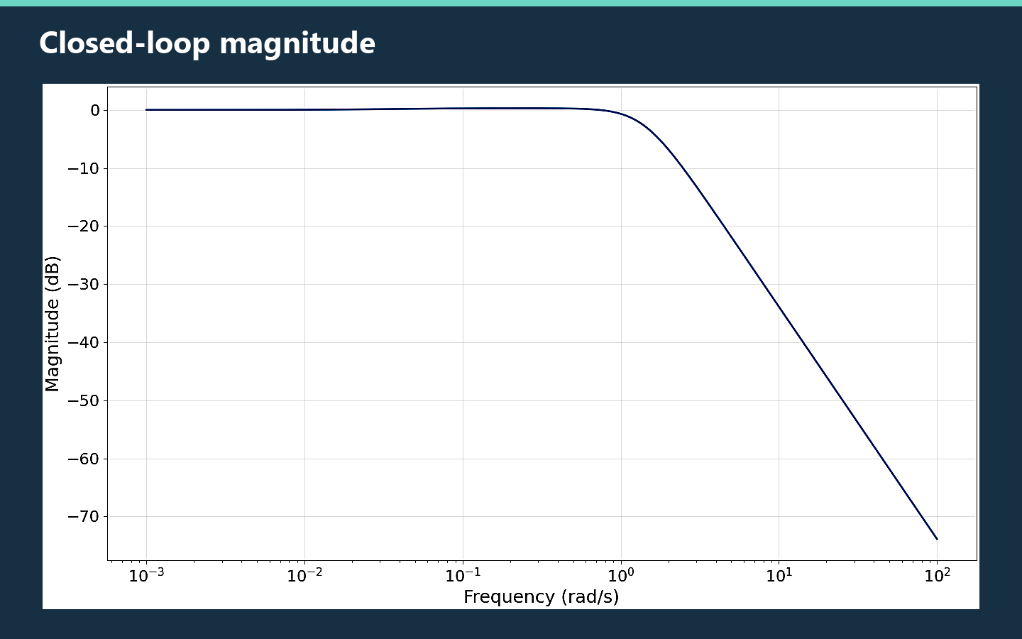
This response describes reference tracking across frequencies.
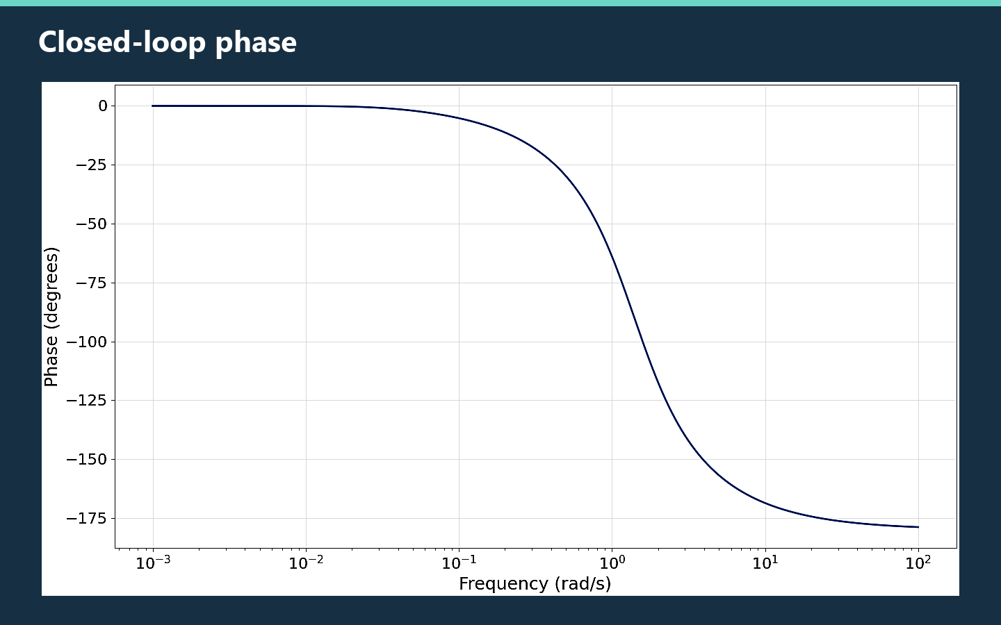
Closed-loop phase is separate from the open-loop stability margins.
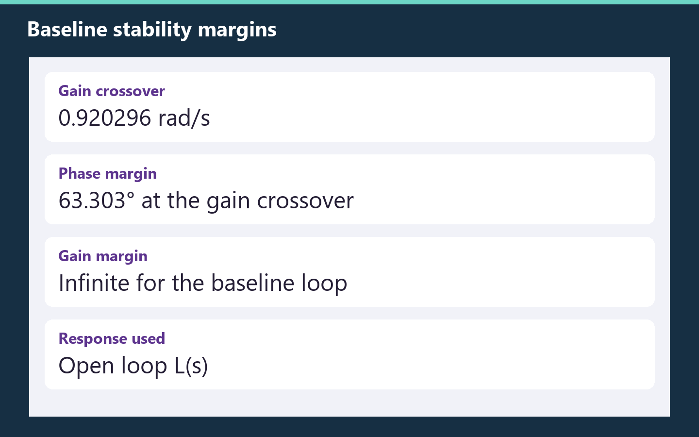
An infinite gain margin indicates no finite −180° phase crossover in the baseline loop.
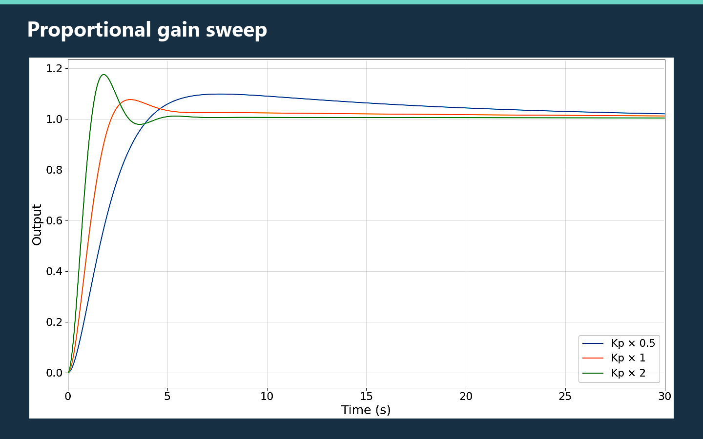
Simulated responses at half, baseline, and double proportional gain with Ki held fixed.
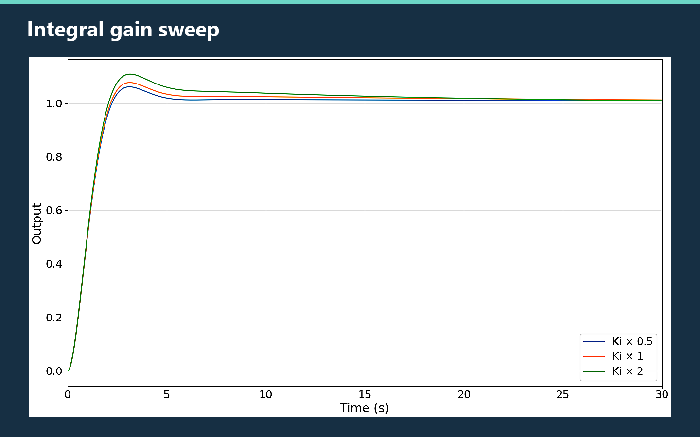
Simulated responses at half, baseline, and double integral gain with Kp held fixed.
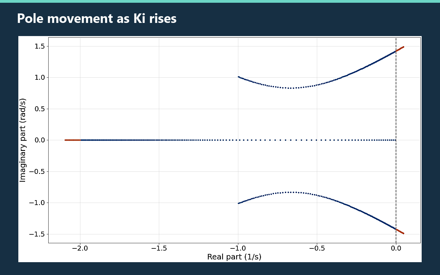
Blue points are stable and orange points lie beyond the Routh boundary.
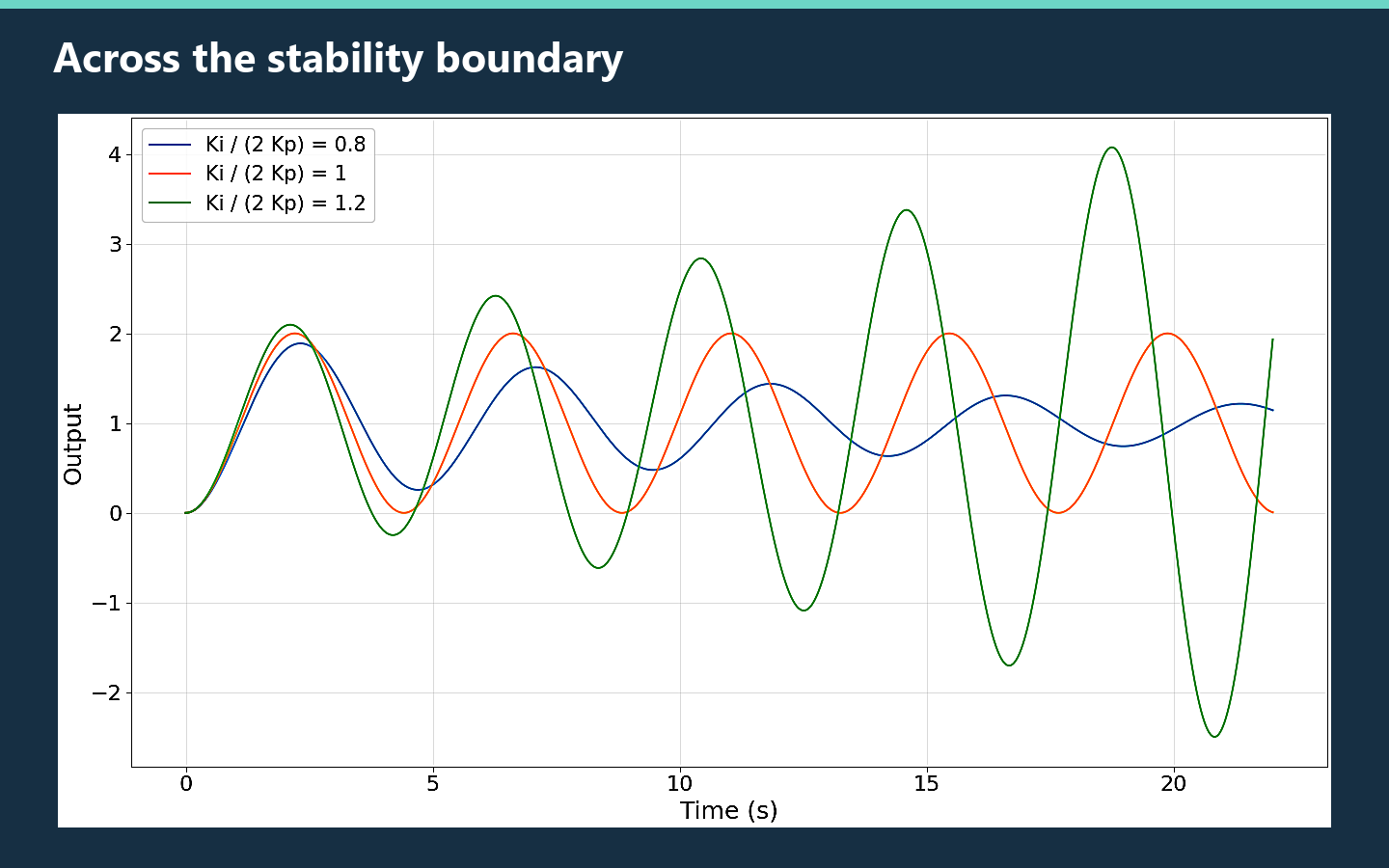
Responses on either side of Ki = 2 Kp illustrate why the strict inequality matters.
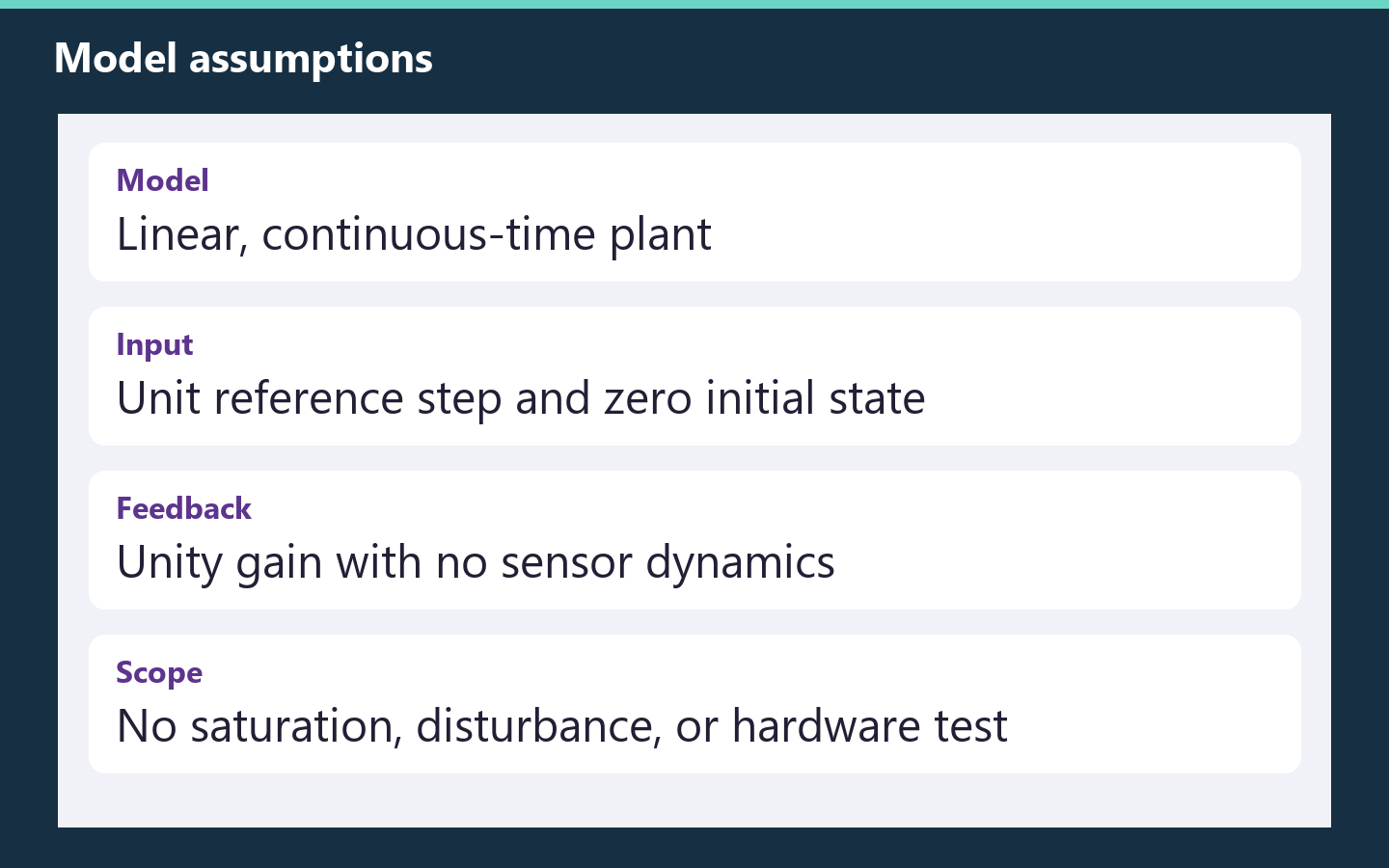
The study uses an ideal continuous-time plant and a linear controller.
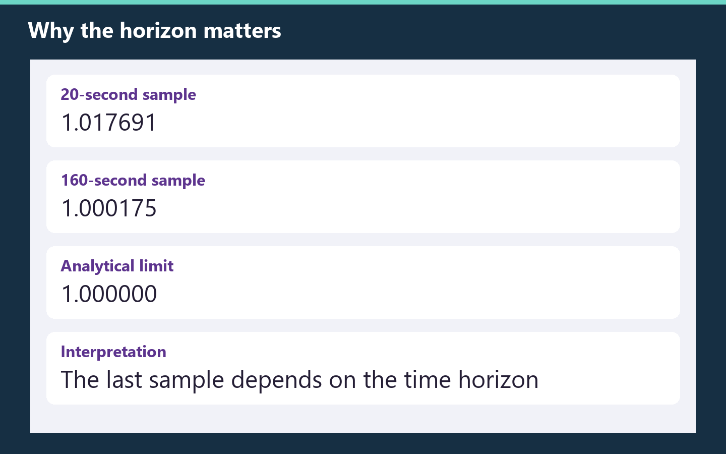
A finite sample and the true steady-state limit answer different questions.
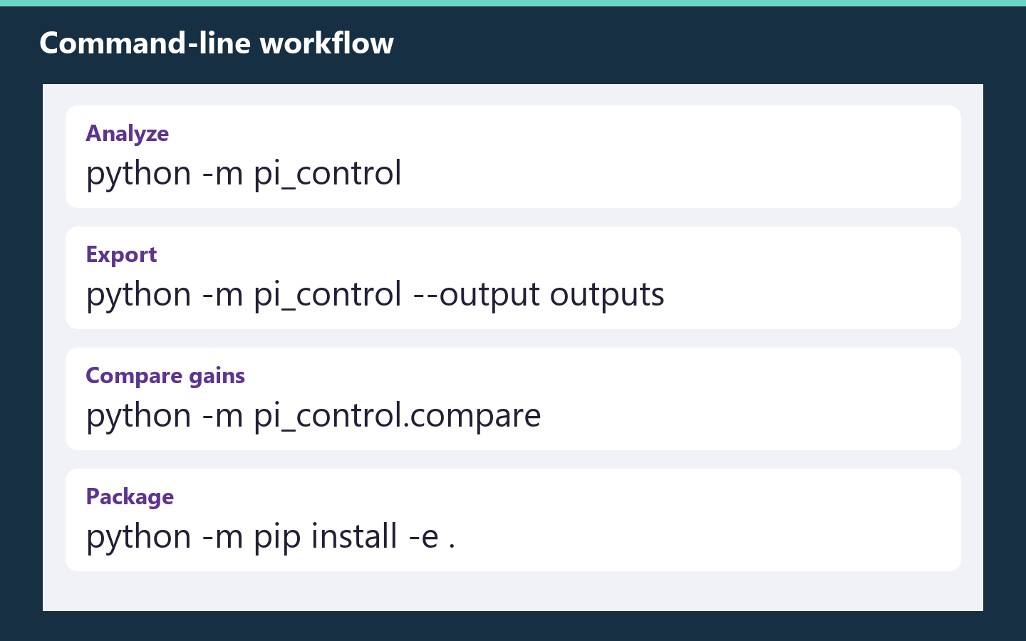
Reproduce the study and export plots or the machine-readable report.
The Python package includes the analysis engine, plot exporters, and a seven-case comparison. The project configuration supports installation and console commands.
python -m pi_control --output outputs/baseline
python -m pi_control.compare --csv outputs/gain_comparison.csv
The first command writes JSON, a time-series CSV, a step-response plot, a pole-zero map, and two Bode plots. The second produces a comparison table. Cases at and beyond marginal stability are included and use blank entries for steady-state metrics.
PI_Control/
├── pi_control/      Analysis and export code
├── docs/            Verification notes
├── assets/          24 figures, previews and site assets
├── pyproject.toml    Installable project configuration
├── requirements.txt
├── index.html
└── README.md
From the repository root on Windows:
python -m venv .venv
.venv/Scripts/python -m pip install -r requirements.txt
.venv/Scripts/python -m pi_control --output outputs
Omit the output flag to print metrics only. Add --help to see the available options.